Network Meta-analysis in R part 1 - by Darko Medin

Network meta-analysis using R part I is the first in the series of tutorials regarding the practical implementations of Network meta-analysis, specifically designed for Clinical Research area. My name is Darko Medin, i am a Senior Biostatistics Consultant and a Meta-analysis expert. Lets start!

I will be using the R programming language[1] and 'netmeta' [2] package to perform network meta-analysis, specifically to discuss how to organize the dataset and create the direct evidence network. I will be using RStudio, Posit IDE for this tutorial [3].

The main goals of this tutorials are to understand the data structuring when conducting the Network meta-analysis and to implement it using R programming language. But its also very important to understand all the context around the Network Meta-analysis implementation.

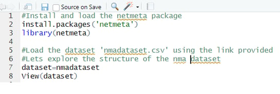
For starters, make sure to install the 'netmeta' by using this code : install.packages('netmeta')

Also you can download the dataset that will be used for this tutorial here :

https://github.com/DarkoMedin/Network-Meta-analysis-1/blob/main/nmadataset.csv

Open the dataset in Rstudio using the Import dataset from text option and set the comma separated delimiters. Make sure to use column names as headers.

Here is how to install the 'netmeta' package and open the dataset in Rstudio

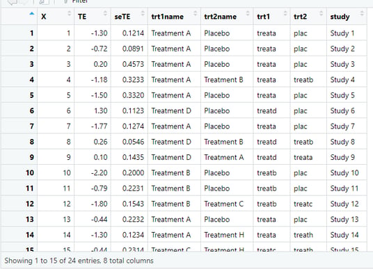
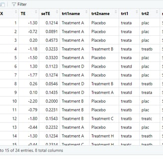
Ok before proceeding, lets discuss how the data for network meta analysis is structured. In the first two rows (excluding variable X which is just index) we can see TE (treatment effect) and seTE (standard error of the treamtment effect).

These are typically present in the pairwise meta-analysis too. But in the network meta-analysis we also need to specify the whole variety of the comparisons instead of single treatment vs control comparison.

The most important columns here are trt1 and trt2 if we want to use short names or trt1name and trt2name if we want to use the full names for the Network meta-analysis. These columns contain the information for the structuring of the direct comparisons of different treatments pairwise and then can be used to construct the network when complemented with the TE and seTE, treamtent effect numerical values. In this tutorial we will use the full names for the esthetics / ease of learning reasons. Finally, in the right side of the image, you can see the column 'study' which would baseically contain the study names, eg. Author et al. but in this case we will use the Study 1 to n as this is a hypothetical practice dataset.

Now lets explore the main network meta-analysis function that will be used. Its called netmeta() and includes specifying exactly the parameters discussed above. So one needs to specify treatment effect point estimate TE, its standard error seTE, Treatment A column and Treatment B column.

Bofore proceeding let me say a few words on the context for the function function we will be using. Whenever we run a function in R, we need to know in detail and have documented what it actually does. The function netmeta() will run the network meta-analysis method as described by Rücker [2012] and Rücker / Schwarzer [2014]. You may read the full documentation on the implementation in these references:

Implementatoin ref 1. Rücker G (2012): Network meta-analysis, electrical networks and graph theory. Research Implementation ref 2. Synthesis Methods, 3, 312–24Rücker G, Schwarzer G (2014): Reduce dimension or reduce weights? Comparing two approaches to multi-arm studies in network meta-analysis. Statistics in Medicine, 33, 4353–69

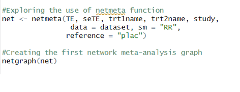
As it can be seen, i also specified the study column, dataset and very importantly sm as 'RR' which stands for risk ratios. Risk ratios or Hazard ratios are the two metrics most commonly used in Clinical trials and Clinical trial Network meta-analysis.

Running a simple netgraph on the net object will produce the following plot :

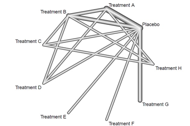
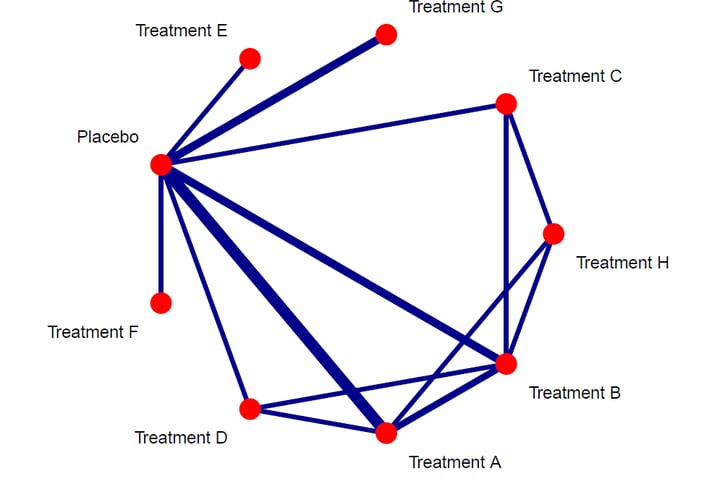
This is the resulting plot. By default the netgraph() function will output the grey 'plastic' plot with edges representing number of studies. Now lets make the plot look more publication ready.

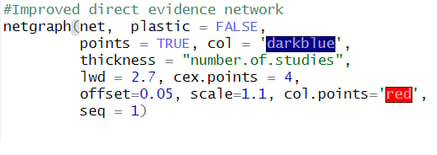
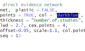
I used the plastic='FALSE' and points='TRUE', to remove the plastic look and add the nodes. Further i set the colors of edges to darkblue and nodes to red. To make sure the number of studies are indeed representing the thickness of the edges, i added this in the code too. Finally, i set the technicalities such as offeset, scale and seq to adapt the labels and the order of nodes. Now run the code and the resulting plot will look more publication ready.

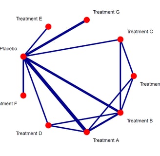
As it can be seen, the plot is now much better esthetically. The plot can now be used for interpretation of the direct evidence potential in the networ meta-analysis. It can be seen that the treatments A, B and G were compared to placebo most frequently in the studies but we can also see the direct comparisons between the treatments too. Finally, we can see which direct comparisons are missing and these will be compared using indirect evidence synthesis in one of the next tutorials in this series.

This is just the first, initial part of conducting the Network Meta-analysis in which the main goal was learning how structure the data, implement the netmeta() function and adjust the direct evidence plot.

In the next tutorial we will explore the additional ordering options within the network and additional plots and outputs used in Network Meta-analysis inference and actual result interpretation. Further in the next tutorials i will also explore the domain specific implementation of NMA in areas such as Oncology and Cardiology.

Thanks for reading and see you in the next tutorial!

by Darko Medin

References :

1. R Core Team (2021). R: A language and environment for statistical computing. R Foundation for Statistical Computing, Vienna, Austria.

2. https://cran.r-project.org/web/packages/netmeta/index.html (Gerta Rücker et al.)